Journal · Rendering
Clouds from orbit
A planet seen from twenty thousand kilometres should look like weather, not like noise. This is how the cloud layer of our procedural planets is built, what went wrong on the way, and what the fixes cost.
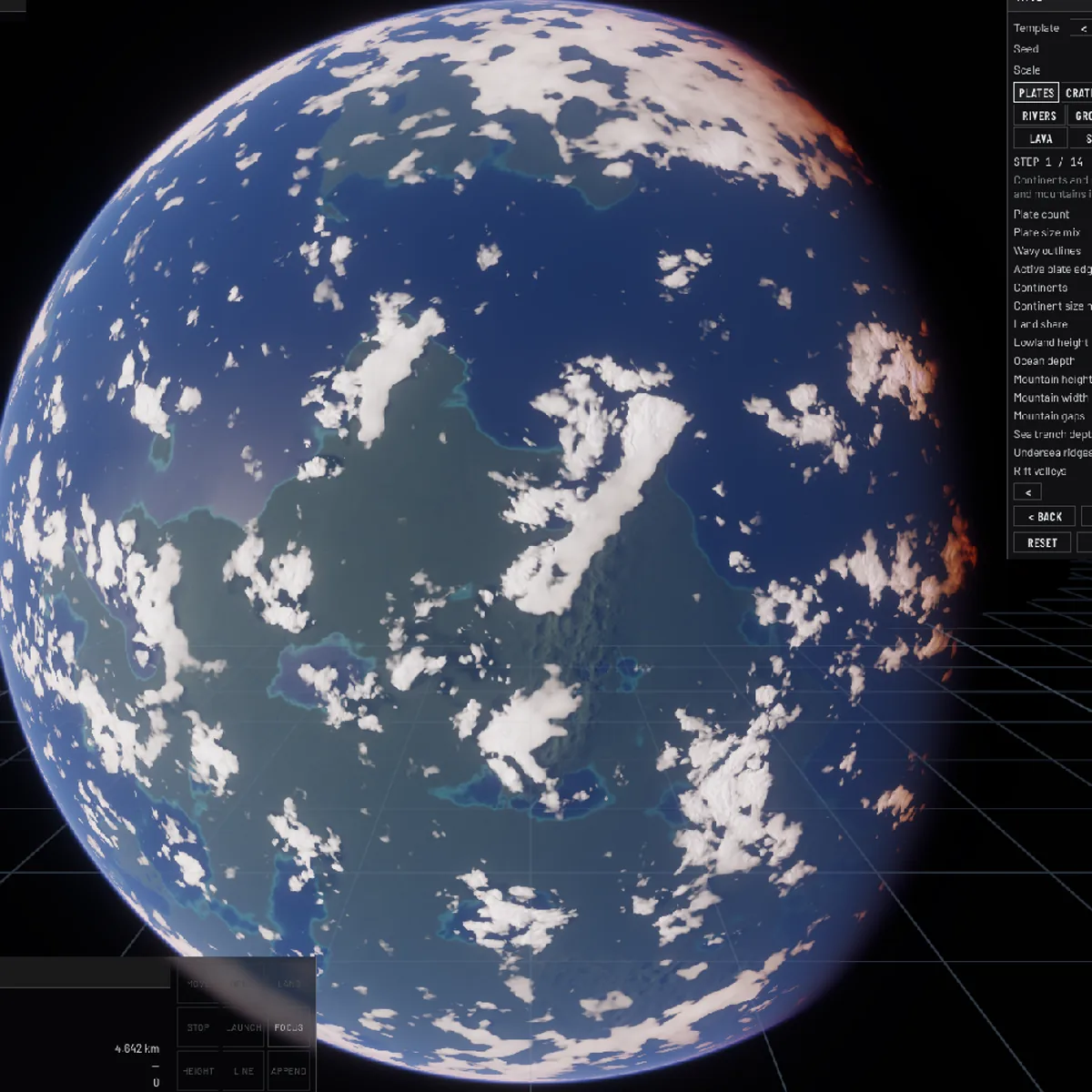
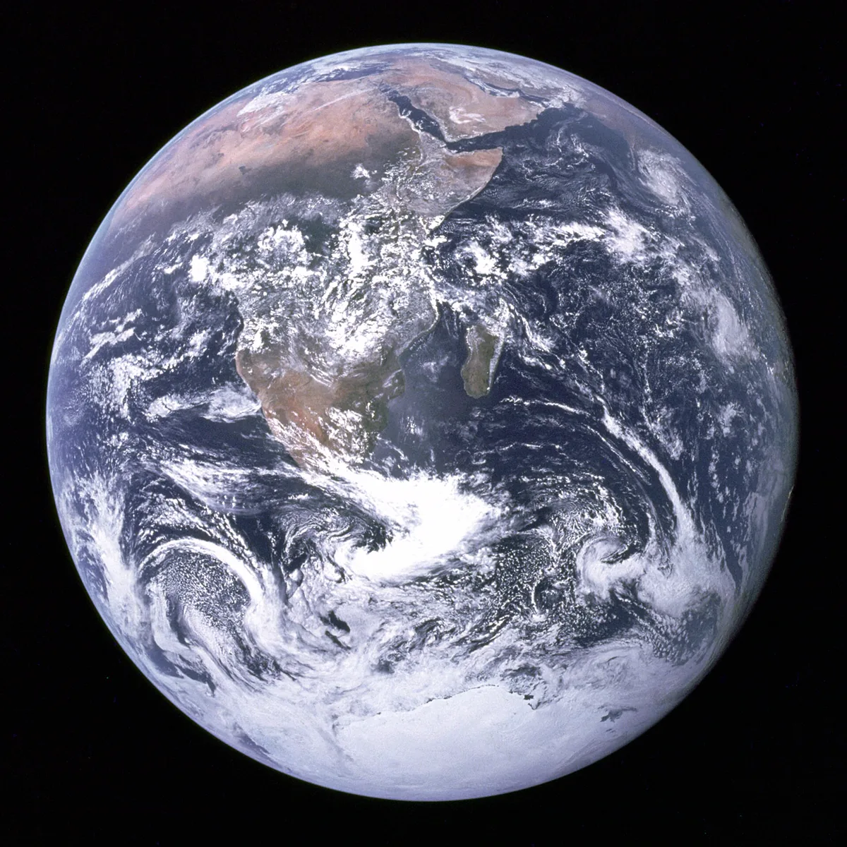
Our planets are generated, not modelled: plates, erosion, climate, rivers and clouds all come out of a bake chain that starts from a seed. The clouds were the part that would not come right. For a long time they were either a soft fog of noise or a field of identical blobs, and every parameter we turned moved the whole planet at once.
What finally worked was splitting the problem by scale. Weather systems are a thousand kilometres across, fronts and cloud fields a hundred, the puffs and fibres you see up close about ten. Each scale needs its own technique, and the three stages have to agree on who decides what. Most of the mistakes below come from one stage doing another stage's job.
1. What orbit shows
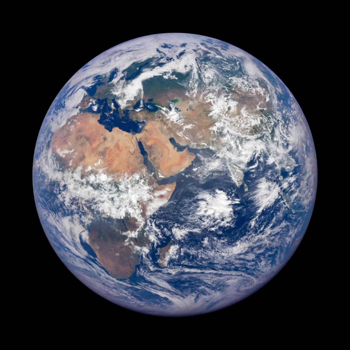
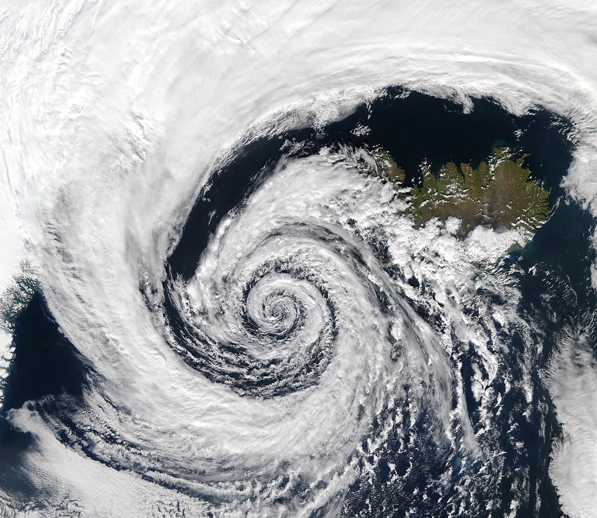
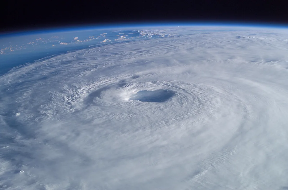
Before writing a line of shader code it pays to look at real pictures for a while. Four things stand out on any true-colour image of Earth, and none of them is noise:
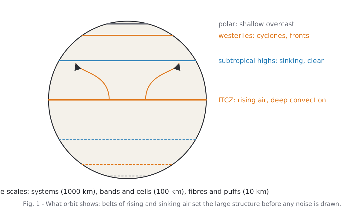
- A band of deep convection along the equator, the intertropical convergence zone, with clear, dry air on both sides of it where the Hadley cells sink.
- Comma-shaped cyclones in the westerlies, each with a dense head and a long tail of frontal cloud.
- Tropical storms as tight spirals with a clear eye.
- Texture that follows the wind: fibres along jets, cellular fields over cool water, streets in the trades.
2. Three stages
The cloud layer is produced in three stages, each one step finer than the last, and none of them waits on the one before it.
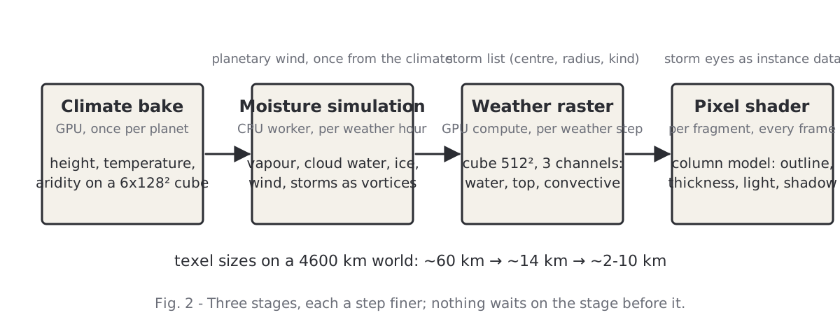
| Stage | Runs on | How often | Resolution |
|---|---|---|---|
| Moisture simulation | CPU worker | once per weather hour | ~60 km (6 × 128² cells) |
| Weather raster | GPU compute | once per weather step | ~14 km (cube 512², 256² for mid-sized discs) |
| Pixel shader | GPU fragment | every frame | ~10 km at a 550 px disc, ~2 km up close |
The simulation is a small moisture model on a cube grid, stepped in weather hours on a worker thread. It knows the climate from the terrain bake, a planetary wind computed once from that climate, and a list of storms that move as vortices. Its output is cloud water, cloud top, convective share and ice per cell.
The raster is a cube map baked on the GPU after every weather step. It takes the simulation's coarse fields and breaks them up below the cell size with noise that follows the simulated wind, then stamps the storm shapes on top. The clouds you see move because this raster moves; the pixel detail does not.
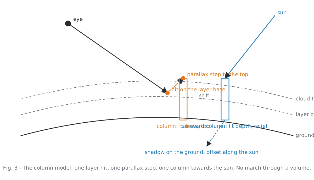
The pixel shader draws a column of cloud for every fragment: where the view ray meets the layer it reads the raster, erodes the outline with fractal noise, computes an optical depth and lights the top. There is no volume march. The camera never goes under the clouds in this game, and a column model turned out to be both cheaper and easier to control than a raymarched volume from orbit.
3. The moisture simulation
The simulation is deliberately not a weather model. Each term exists because it makes clouds sit where they would on Earth. Per cell and per hour: vapour and cloud water are carried in with the wind (a semi-Lagrangian step backwards along the flow); the surface pulls the air towards its climatic humidity, faster over sea; lift from slopes, convergence, storms and wandering disturbances lowers the saturation, and whatever vapour is now above it condenses; warm, unstable air turns lift into convection, which lofts water into ice that the upper wind spreads; rain removes water, ice decays over a day.
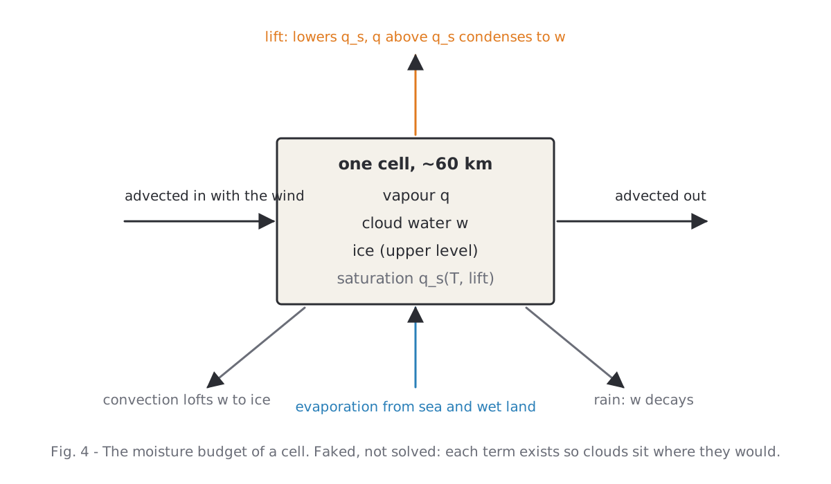
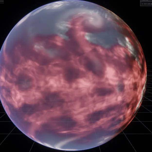
First lesson. Humidity alone produced an even field of puffs from 30° S to 30° N. The sub-grid cloud, the part of a cell that is cloudy without the whole cell saturating, has to follow the lift: sinking air thins it, rising air feeds it. With that single factor the ITCZ appeared, the subtropics cleared (about half the cells clear at ±30°) and the air behind fronts opened up.
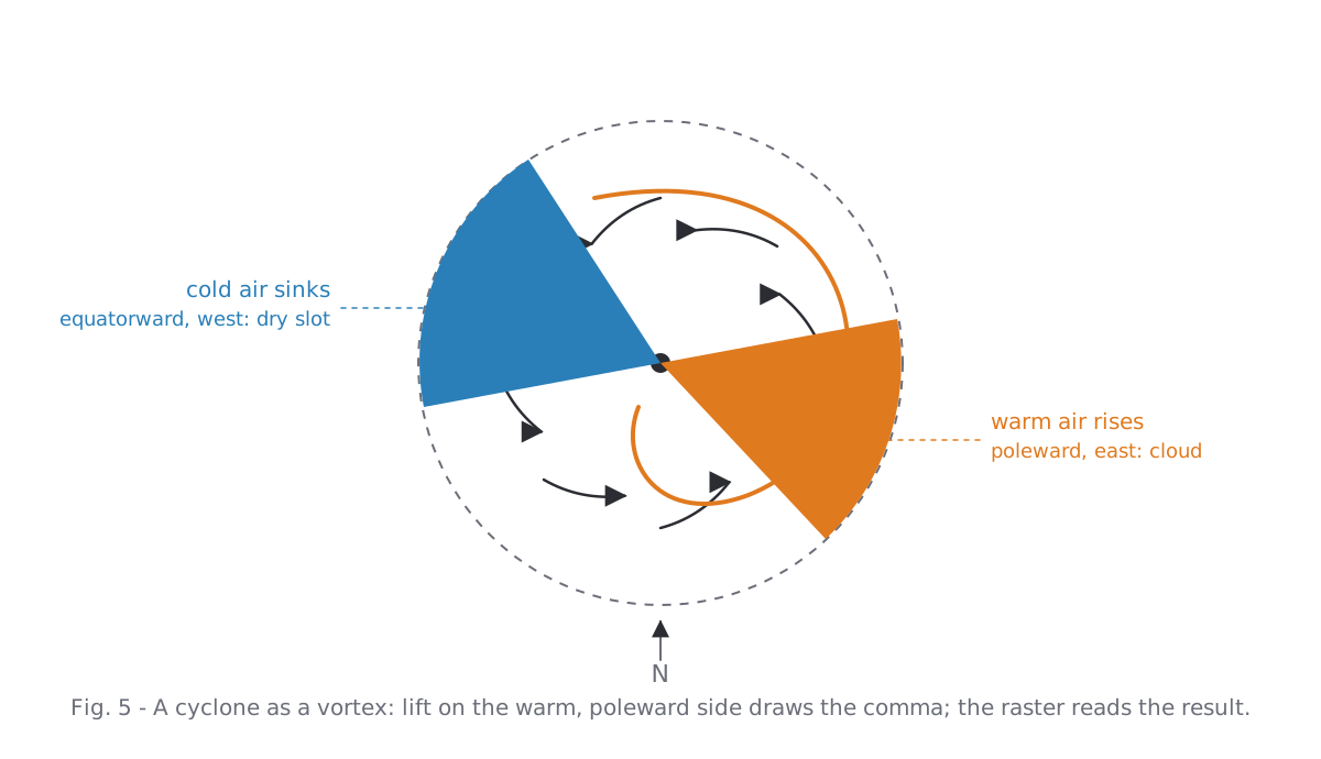
Storms are vortices in this model. A cyclone turns the air about its centre, draws it in, lifts it in the core and, on its poleward eastern side, lifts the warm air that becomes the comma; cold air sinks on the other side and clears the dry slot. A tropical storm is the same vortex with a smaller core, faster winds and an eye in which the air sinks.
4. The weather raster
Sixty-kilometre cells are far too coarse to look like cloud. The raster's job is to invent the structure between the cell size and the pixel in a way that still belongs to the simulated weather. Three ideas carry it.
Noise along the streamline
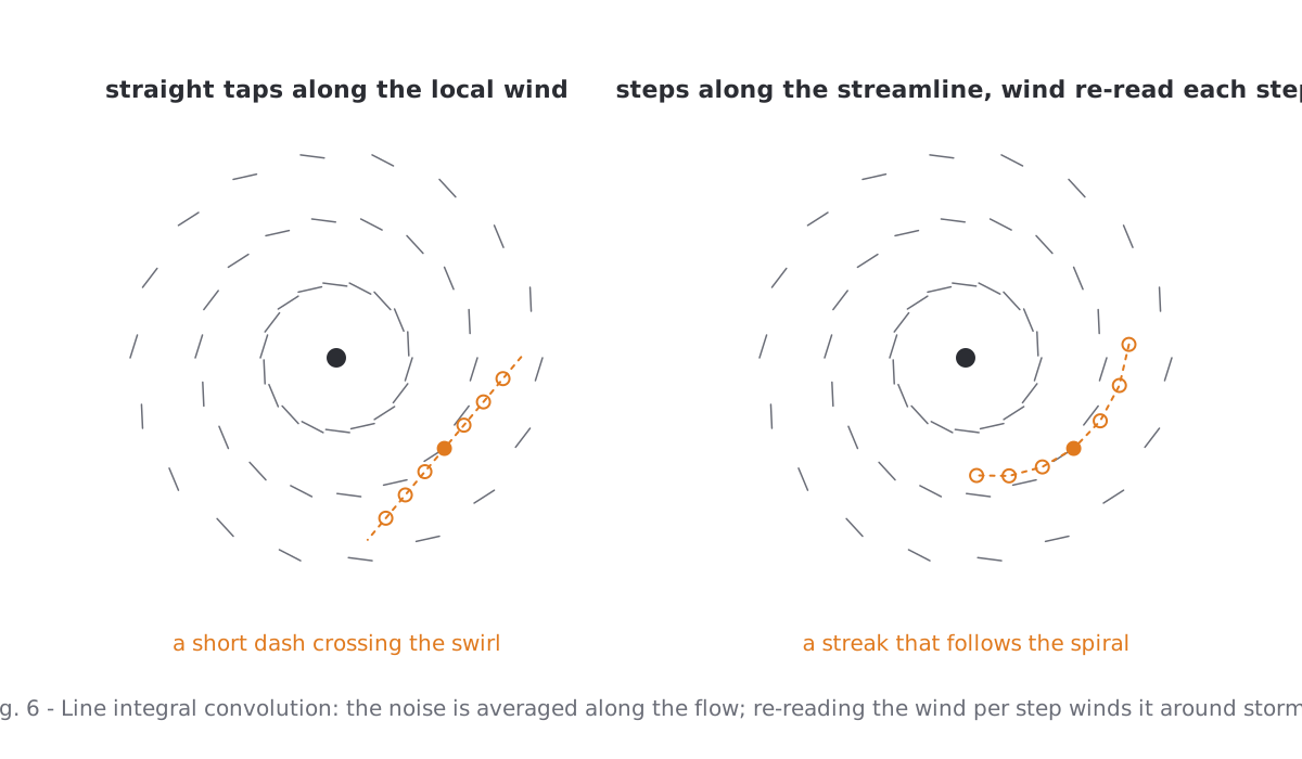
Plain noise multiplied onto the water gives blotches. Noise averaged along the wind gives streaks. The first version averaged a few taps along the local wind direction and drew short dashes that cut across every swirl, because the wind turns within the length of a dash. The fix is textbook line integral convolution: walk a few steps along the streamline, re-reading the wind at every step, and average the noise along that path. Streaks now wind around storms and bend along fronts.
Multiply exponentially
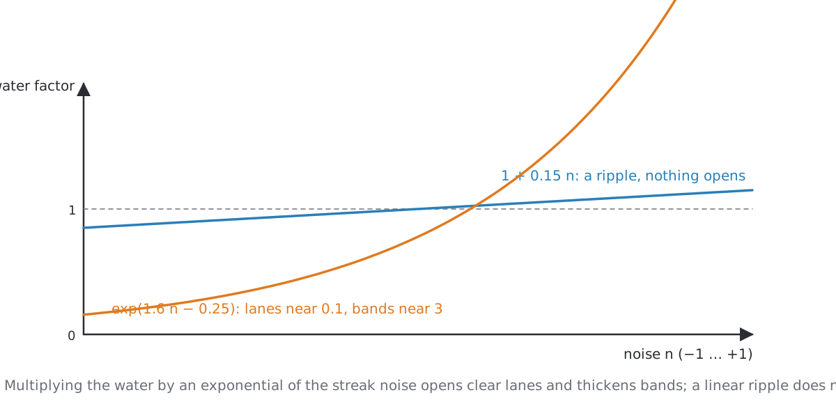
A linear modulation such as water × (1 + 0.15 n) is a ripple; you cannot see it from orbit. Using the noise as an exponent, water × exp(1.6 n − 0.25), opens real lanes where the noise is low and thickens bands where it is high, which is what the photographs show between the cells of a field.
Respect the texel
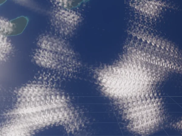
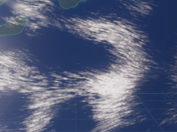
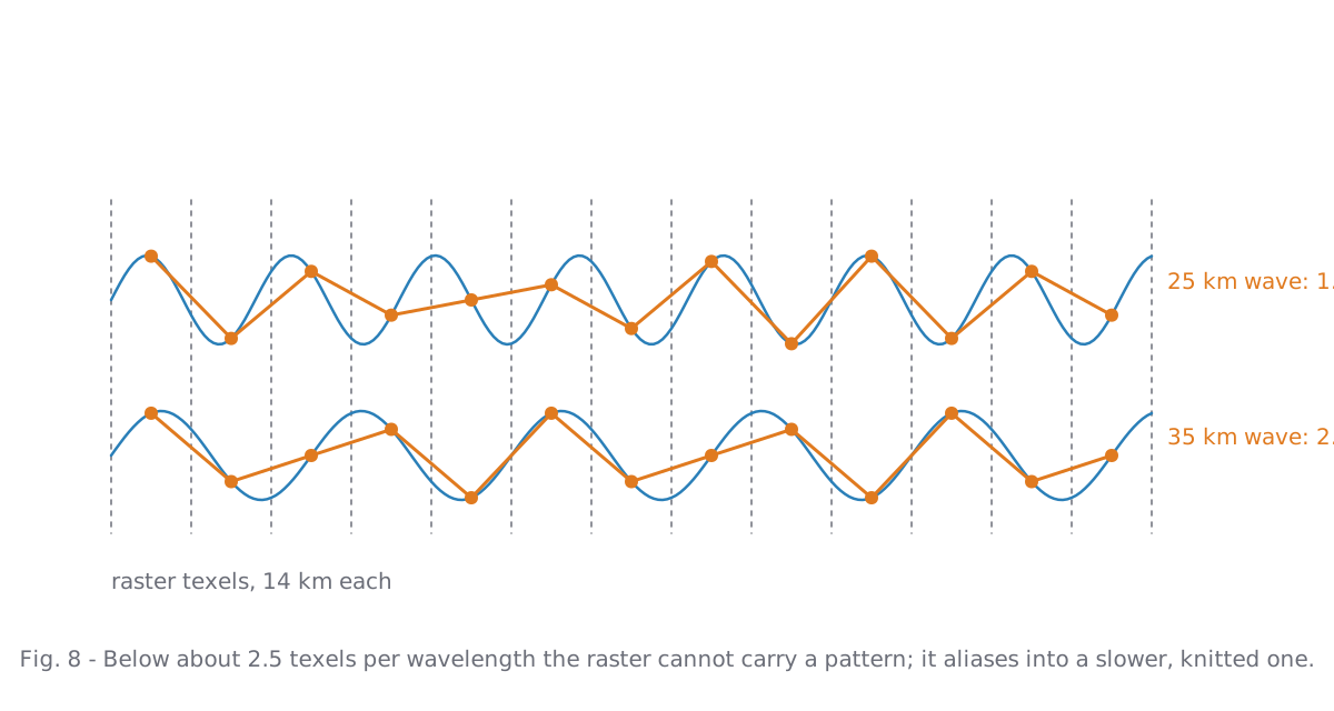
The first attempt at fibres used one noise octave of 25 km wavelength on 14 km texels, with taps 85 km apart. It produced a knitted grain and, closer in, a herringbone. Both are aliasing: a pattern shorter than about 2.5 texels cannot be carried by the raster and folds into a slower one, and taps spaced further apart than the wavelength stack shifted copies of the pattern. The detail is now a 1/f octave series from 220 km down to 2.5 texels, bent by a domain warp, evaluated once per texel.
Storm bands in kilometres
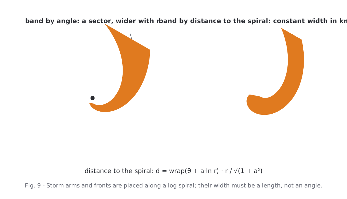
Spiral arms and fronts are placed along a log spiral around the storm centre. The obvious way to draw a band around that curve, a function of the angle θ + a·ln r, produces a sector that widens with the radius: at the end of a 1700 km cyclone the "band" was a fan a thousand kilometres wide. A band needs a width in kilometres, which is the distance to the spiral, wrap(θ + a·ln r) · r / √(1 + a²). The width then swells and narrows along the band with a slow noise so it does not read as a drawn tube.
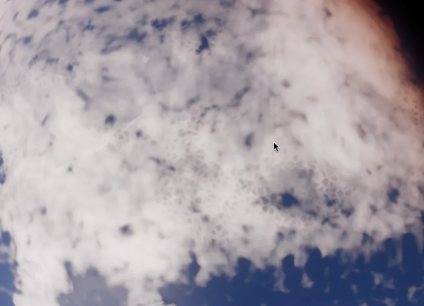
One more thing the raster must not do: anything smaller than about four texels. A Voronoi pattern of open cells at 70 km looked plausible from far away and became a honeycomb of hexagons as soon as the camera came closer. It went out again.
5. The pixel shader: erosion, not a threshold
This is where most of the time went, and the mistake is worth describing in full because it looks like a tuning problem and is not one.
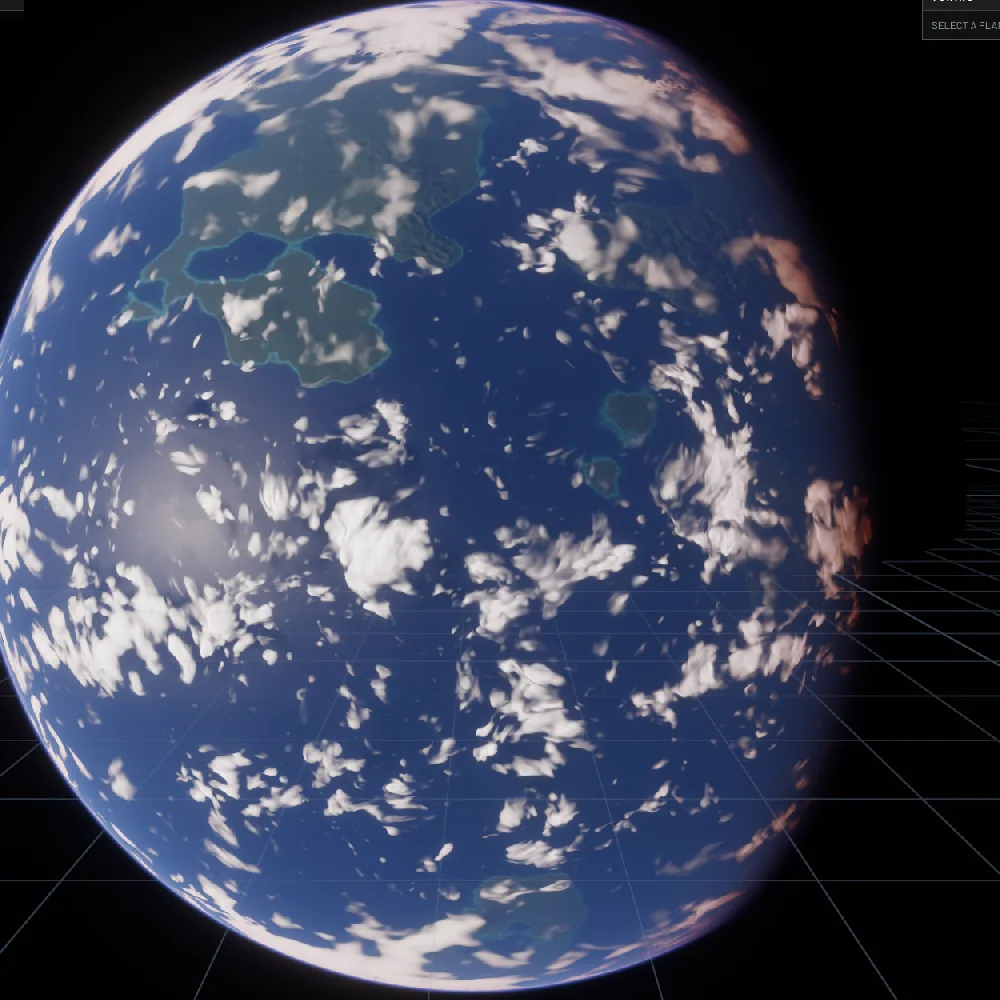
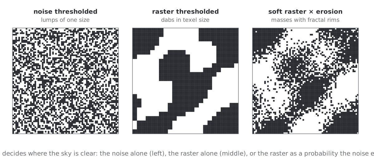
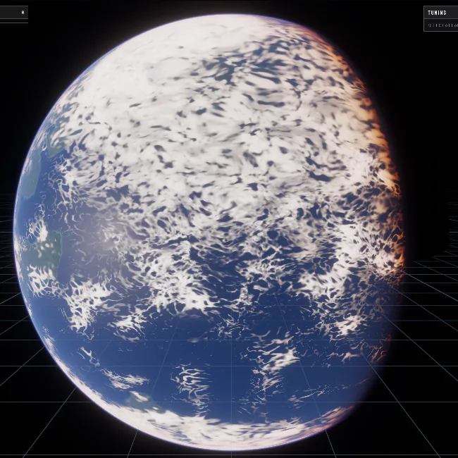
The pixel shader builds a fractal noise (an fBm of gradient noise, up to twelve octaves) and decides from it whether a pixel is cloudy: compare the noise to a threshold derived from the raster's coverage, ramp the edge a little, done. That is how most procedural clouds work. From orbit it fails in a specific way. The threshold is nearly the same everywhere, so the largest octave of the noise decides the shapes everywhere, and the largest octave has one size. The planet was stamped with lumps of that size, whether the raster said "storm" or "clear".
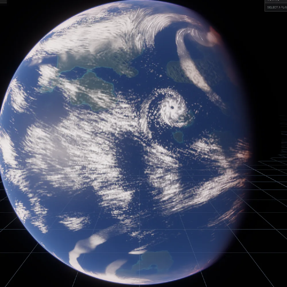
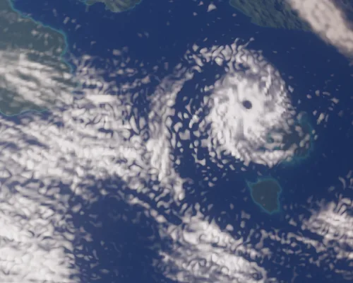
The first reaction was to let the raster decide instead: clear the sky in the raster, use the pixel noise only to texture what is left. That removes the lumps and replaces them with something worse. The raster has 14 km texels and is sampled bilinearly, so every cloud edge became a soft blob the size of a texel. Paint dabs.
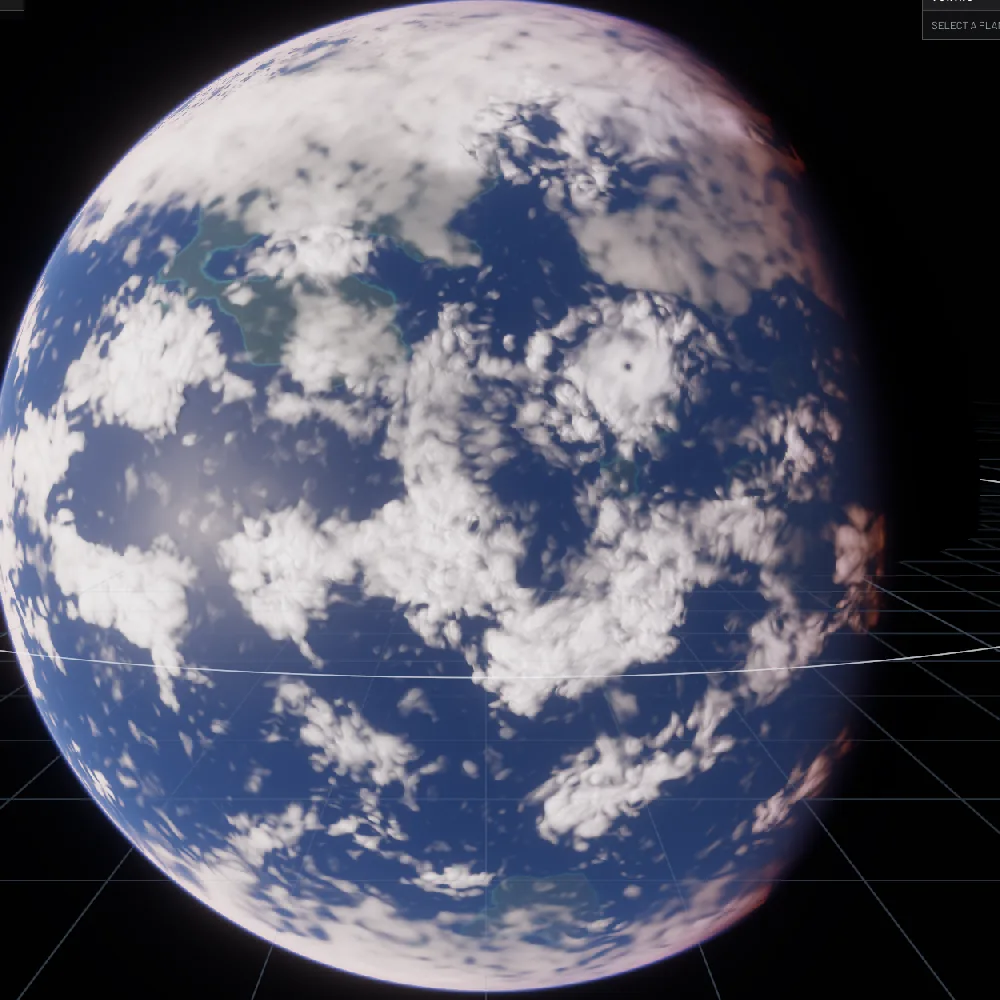
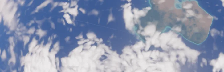
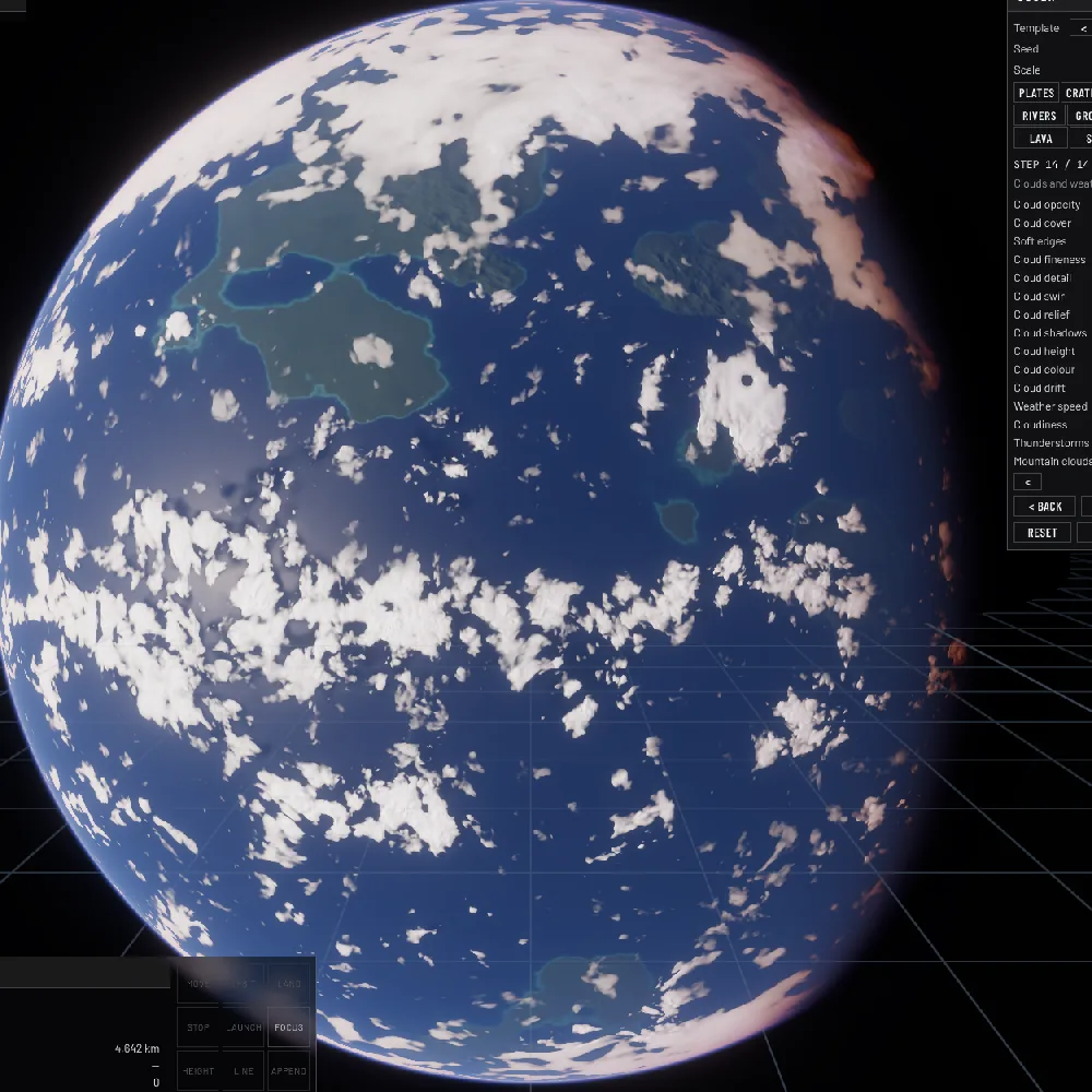
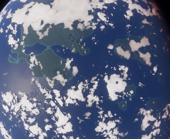
The version that works is the one volumetric cloud renderers have used for years, transposed to a layer: the raster is a probability of cloud, soft and continuous, and the fractal noise erodes the cloud out of it. Where the raster says 0.9 only the finest octaves nibble at the rim; where it says 0.4 the field breaks into specks; where it says 0.05 nothing survives. Large masses stay large with fractal rims, and medium cover looks like medium cover.
The numbers behind it
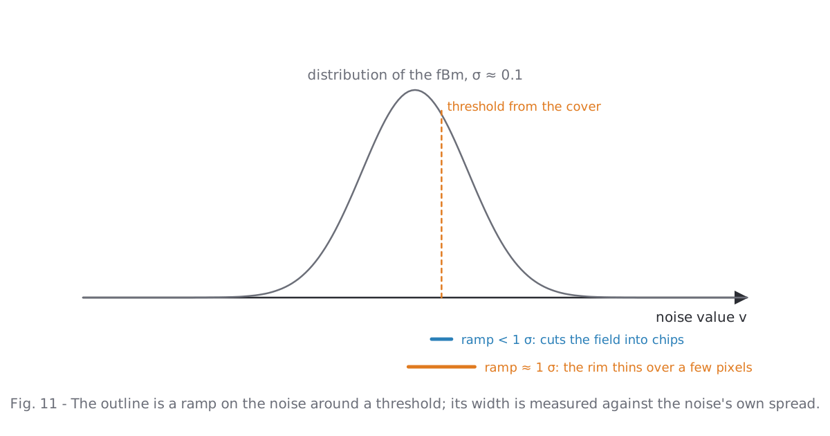
The raster's water w becomes a sky cover c = 1 − exp(−w·s), with a spread s of 3 for sheets and 1 for convective cloud (towers leave gaps between the puffs, sheets close up). The cover sets a threshold on the fBm, t = 0.5 − 0.6·(c − 0.5), so that about the share c of the noise lies above it. The outline is a smooth ramp around t. Two details matter:
- The ramp must be measured against the noise's own spread. Our fBm has a standard deviation near 0.1; a ramp much narrower than that cuts the field into chips, a ramp much wider makes grey veils. A quarter of the softness control, about one σ, was the sweet spot.
- Octaves finer than the pixel fade out to avoid shimmer as the planet turns, and what they would have contributed to the spread is added back to the ramp width. Without that, far planets either lose their clouds or close up, because the threshold then meets a smoothed field.
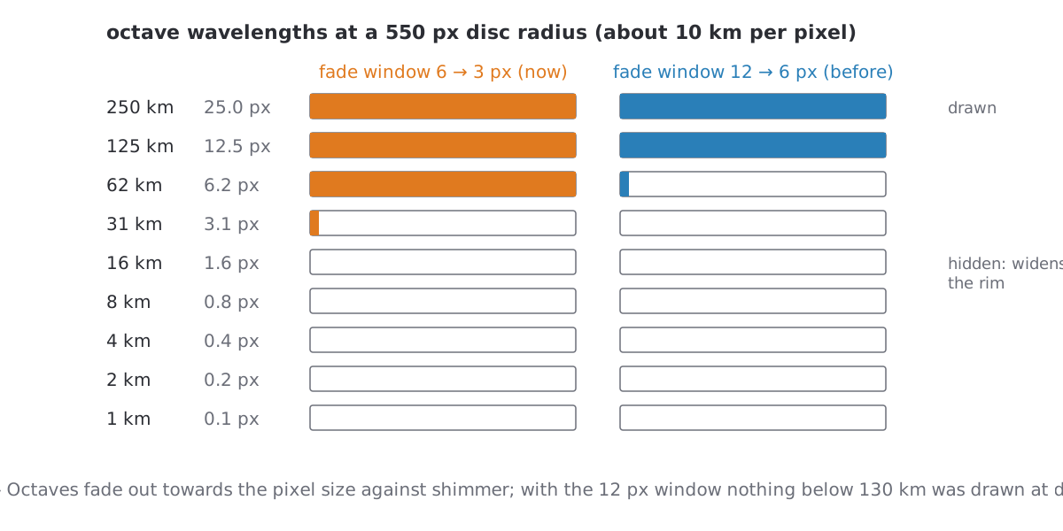
The fade window itself was a trap. Against shimmer we faded octaves from twelve pixels of wavelength down to six. At a 550 px disc one pixel is ten kilometres, so nothing below 130 km was ever drawn, and every cloud was a soft dab regardless of what the raster said. The window is now six to three pixels; the measured flicker of a turning disc went from about 0.6 % to 1 % of pixels, which is invisible.
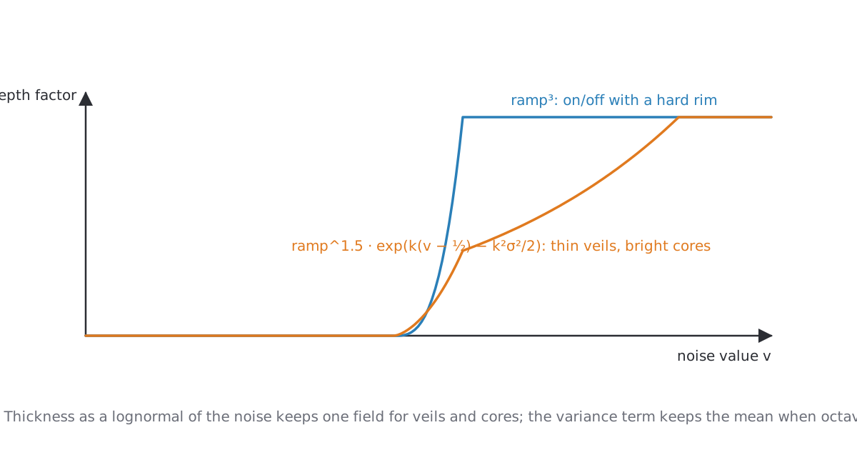
Thickness is a separate field from the outline. The first version used the cube of the edge ramp, which gives on/off cloud with a hard rim. Now the thickness is lognormal in the noise, exp(k·(v − ½) − k²σ²/2), with the variance term keeping the mean thickness when octaves fade. Thin veils and bright cores come from the same field, and no cover cuts to a binary edge.
A small one to finish the section: convective cloud folds the noise (|n|) for billowy heads. Folded the wrong way round, the zero lines of the noise became bright veins through every cloud. It took a close look to see, and a sign to fix.
6. Light on the deck
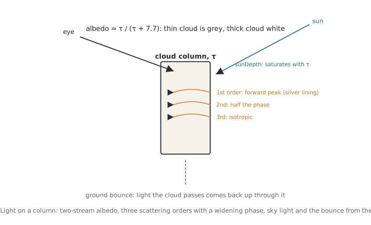
A column's brightness follows the two-stream albedo of a cloud layer, τ / (τ + 7.7): opacity alone saturates at τ ≈ 3 and made thin and thick cloud equally white, so masses read as flat patches. Sunlight enters the column at a depth that saturates with τ, scatters in three orders whose phase widens from a forward peak to isotropic, and is joined by sky light and by light the ground sends back up through the cloud. That last term matters more than it sounds: without it, thin cloud over snow was a grey stain darker than the snow next to it.
Relief from two columns
The towers and furrows you see on a deck are not geometry. A second column is read a few kilometres towards the sun; where its top is higher than ours we are in its shadow, where it is lower we are a sunward slope. One multiply on the direct light.
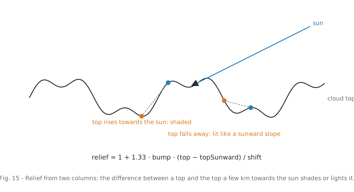
Second lesson. This relief depended on the sun's height. The sunward shift grew with 1/μ of the sun, so under a low sun the comparison column sat far away and the differences averaged out; the self-shadow saturated as well. Clouds under a high sun had furrows, clouds towards the poles and the terminator were flat white. Physically defensible, visually wrong: the same structure everywhere looks better. The relief and the self-shadow are now computed as for a sun at least 0.55 above the layer, and the sky light carries half the relief.
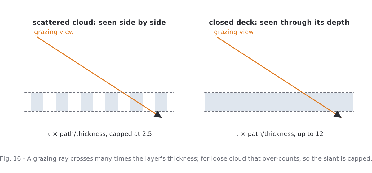
A related one: the path through the layer. A grazing ray crosses many times the layer's thickness, and the first version multiplied τ by that factor, up to twelve. Near the limb every cloud became opaque, the albedo saturated, texture and translucent rims disappeared. Scattered cloud is seen side by side, not through twelve layers of itself; the factor is now capped at 2.5.
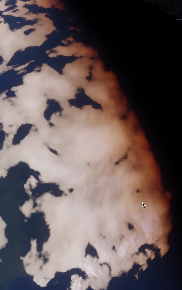
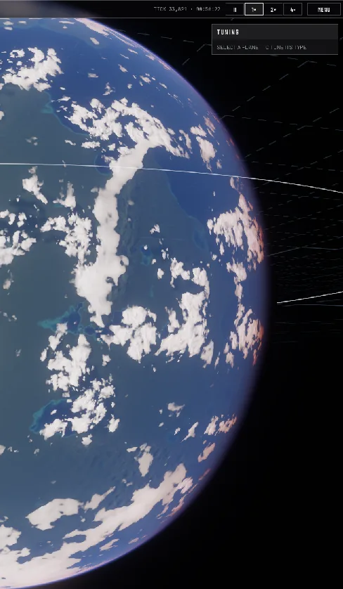
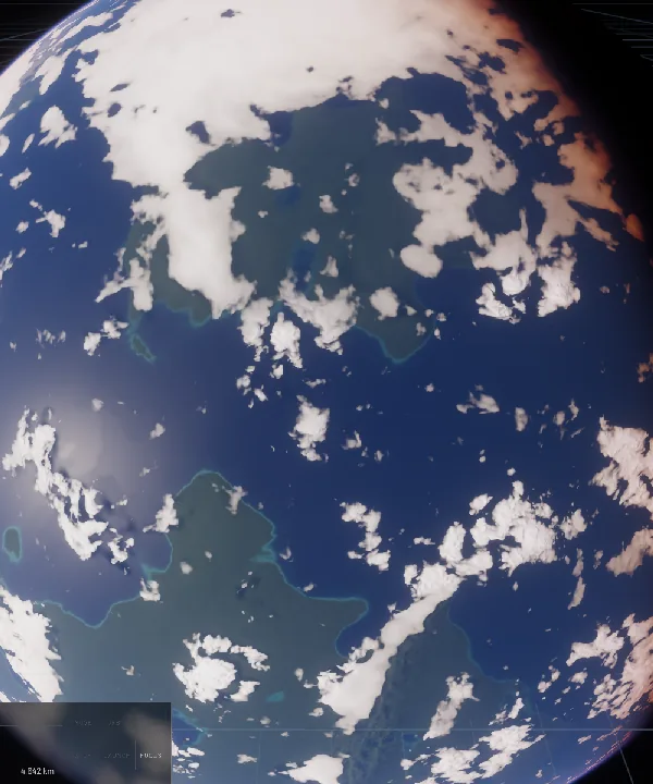
And one that was a design choice rather than a bug: only convective cloud had the billowy texture; sheets were flatter by design. On a planet that meant structure near the equator of earth-like worlds and smooth decks at the poles, over mountains and on every cold or dry world. We dropped the distinction. Polar and orographic cloud is less tower-like in reality, but from orbit it is anything but smooth.
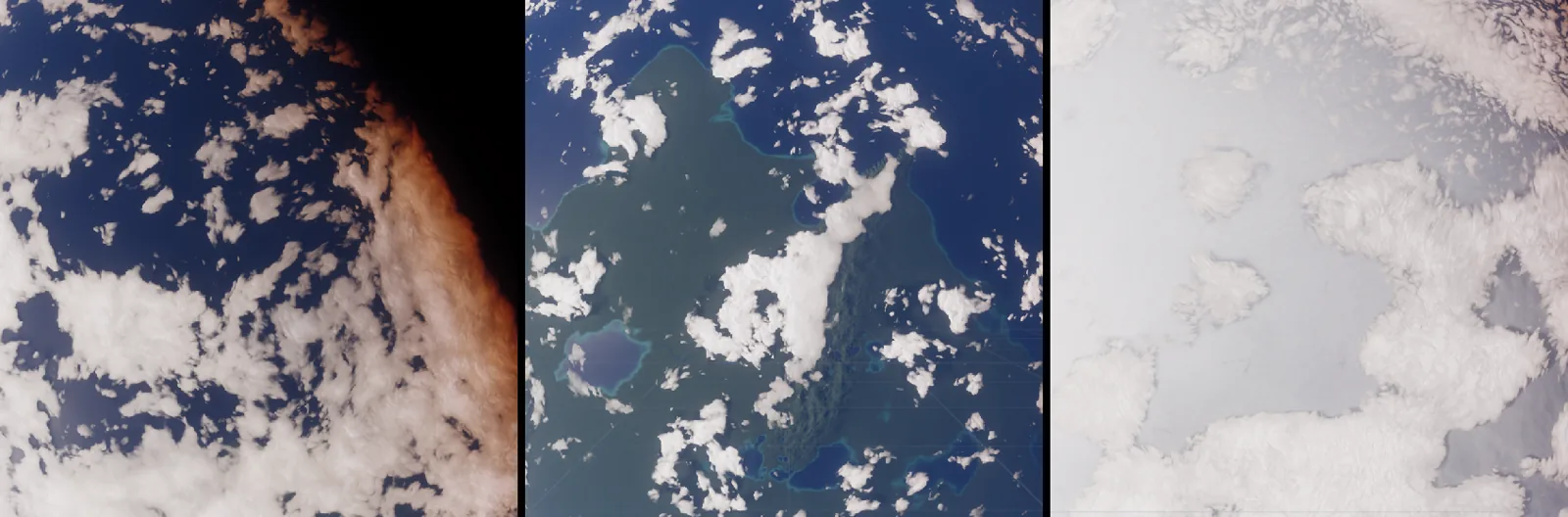
7. The eye of the storm, three times
The eye of a tropical storm is small, about 45 km across, and it is the one place where a viewer will zoom in. It took three rounds.
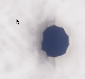
Round one drew it in the raster as a clear circle with a dense wall around it. On 14 km texels a 45 km circle is an octagon, and the bilinear filter does not hide that. Widening the edge made it a rounder octagon.
Round two found a bright streak next to the eye that no amount of widening touched. Its cause was the parallax step of the column model: the view ray is first intersected with the layer base, then stepped to the cloud top read there. The eyewall raised the top to twelve kilometres and the eye dropped it to one, so along the rim the step jumped by a hundred and fifty kilometres sideways and sampled cloud that was not under the pixel.
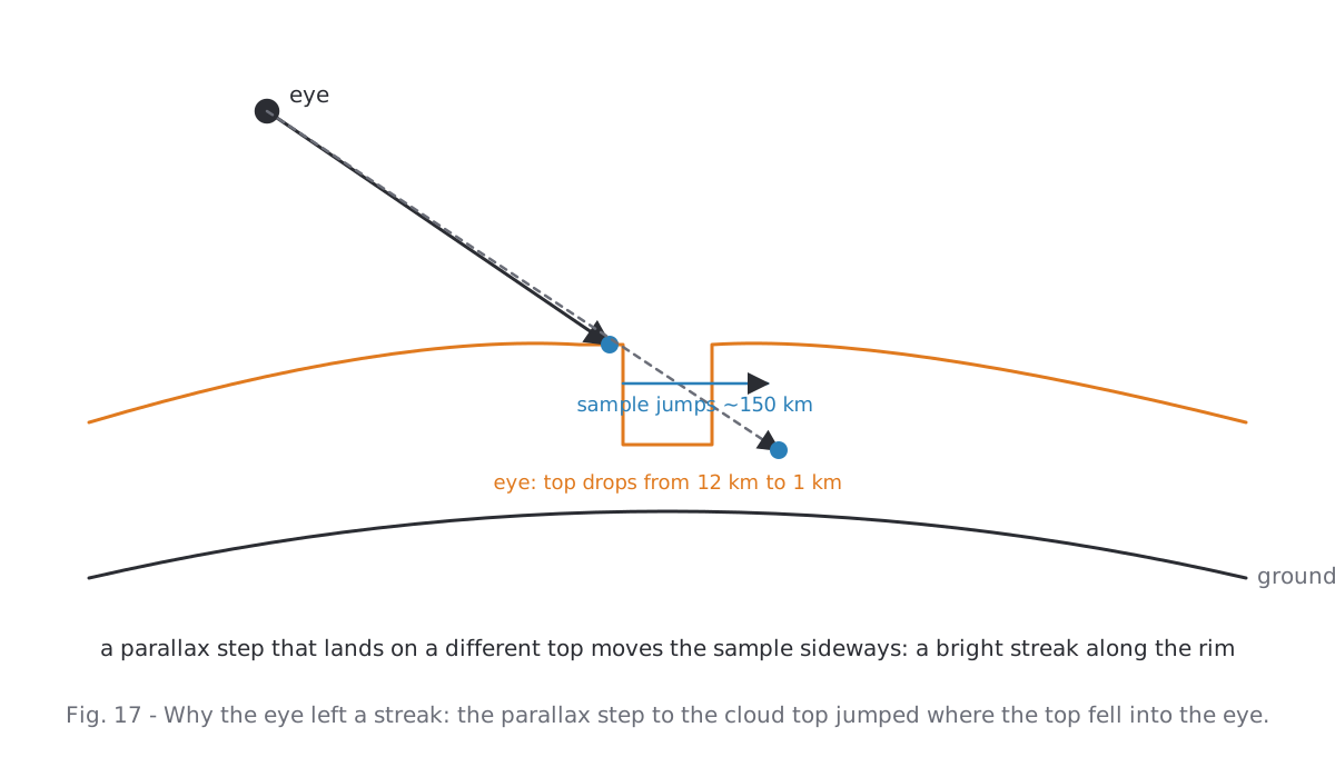
Round three took the eye out of the raster altogether. The storm list already exists on the CPU; the four strongest eyes go into the planet's instance data as centre and radius, and the pixel shader cuts them analytically, once per pixel on the layer direction, as a factor on both columns. Cut inside the raster lookup instead, the parallax-shifted and the sunward column each cut their own circle: a double contour. The rim wavers by three lobes that turn with the drift, because a perfect circle reads as a drawn one.
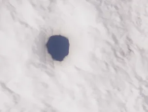
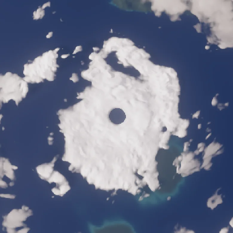
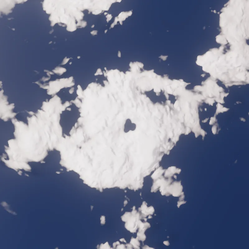
The rule that came out of it: anything smaller than about four raster texels does not belong in the raster. Either it is analytic in the pixel shader, or it does not exist.
8. The air, briefly
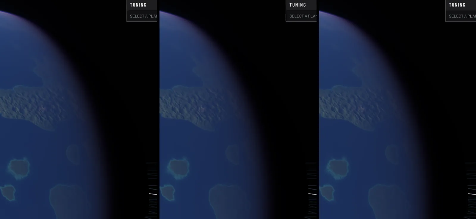
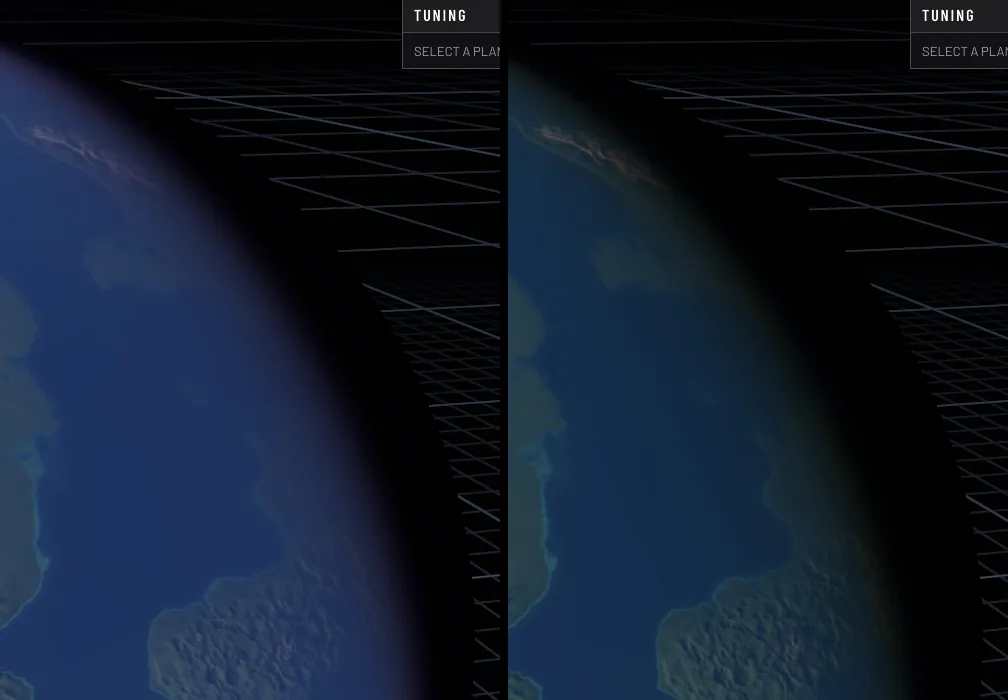
The clouds sit inside a physically based atmosphere after Hillaire's model, with transmittance, multiple scattering and sky irradiance tables baked per planet type. The view ray used to be marched through it, eight to thirty-two steps per pixel with three table lookups each. It now reads a fourth table, the scattering along any ray through the shell after Bruneton, four parameters packed into one 2D texture. A segment of air between two points is S(a) − T(a,b)·S(b); a segment that ends on the ground or at the top of the shell needs one lookup. The highest quality tier still marches, but only on segments a moon's shadow can reach. The image difference to the full march is 0.6 of 255.
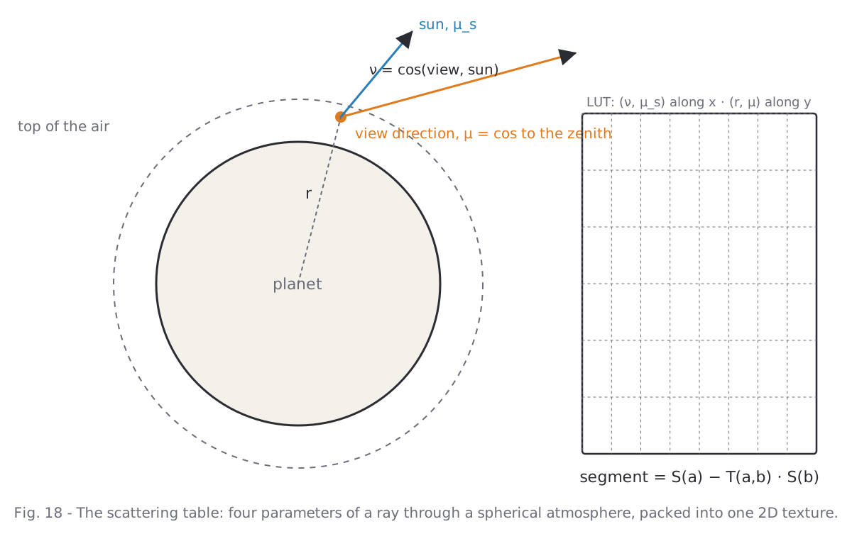
The cheapest model was supposed to be a one-point approximation per segment. It was barely cheaper than the table and drew an orange rim at the limb and a grey glow over the night side, because one sample cannot be both where the light is gathered and where it is shaded. The minimal tier now reads the same table at its nearest altitude slice instead.
9. What it costs
All numbers are GPU milliseconds of the planet pass for an earth-like planet filling a 550 px radius, on a desktop GPU, before and after this work. The lower tiers draw a static deck: the live clouds of one moment baked into a cube with every mip evaluated at its own texel size, then only turned with the cloud spin. The weather of that planet rests until a control or the climate changes.
| Quality | Before | After | Clouds | Air |
|---|---|---|---|---|
| Minimal | 1.35 ms | 0.60 ms | static deck | table, nearest slice |
| Low | 1.42 ms | 0.68 ms | static deck | table |
| Medium | 1.99 ms | 1.56 ms | live, 6 octaves | table |
| High | 2.63 ms | 2.71 ms | live, 8 octaves | table |
| Ultra | 3.08 ms | 2.75 ms | live, 12 octaves | table, march in eclipses |
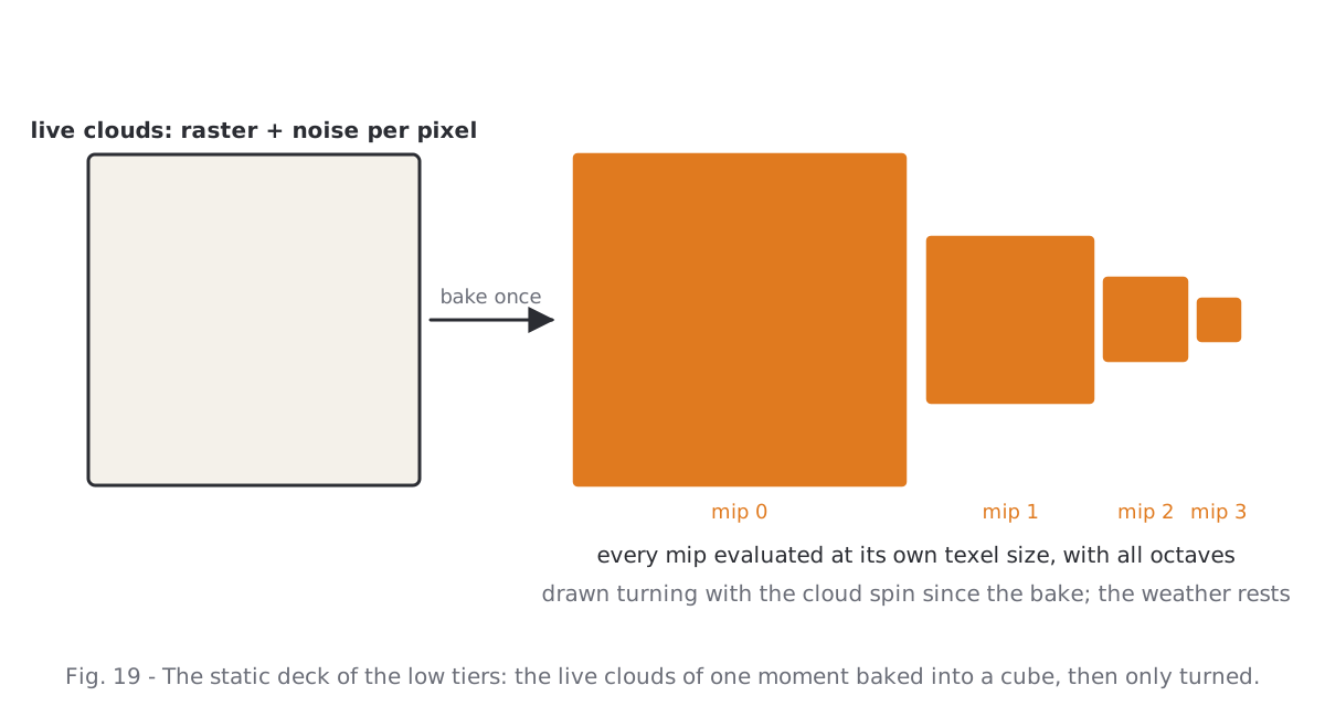
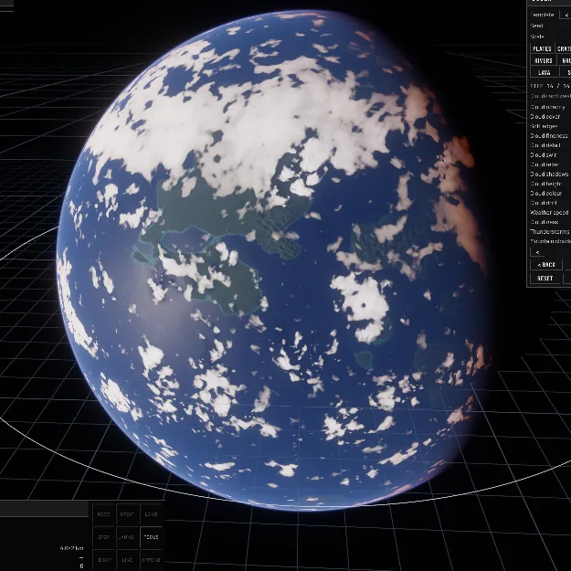
Bakes are cheap by comparison: the weather raster costs under a millisecond per cube face at 512², once per weather step; the static deck about a millisecond per face, once; the scattering table under a millisecond, once per planet type. The high tiers did not get cheaper, because they now draw three or four real octaves where before they drew one; the low tiers halved.
Two things that were tried and taken out again, so nobody tries them twice: a cold front as a lifting line in the simulation, which turned every cyclone into an oversized, identical comma; and cloud streets in the trades, which doubled the raster bake for an effect invisible from disc distance.

10. Working against photographs
Every round of this followed the same loop: pick a real image of the subject, render the same subject at the same scale, put them side by side, name what differs, change one thing. The loop failed exactly when it was shortened. Judging from downscaled contact sheets hid the leopard pattern for a whole day; the raster's hexagons only showed in a close-up. Full resolution, a crop, and the reference next to it, or the comparison is not worth making.
What is still missing against the Apollo picture: the long frontal bands of the westerlies, which have to come from the simulation rather than from drawing, and the cellular fields over cool coastal water. Both are on the list.
Reference photographs: NASA (Apollo 17 AS17-148-22727; DSCOVR EPIC; MODIS Terra; ISS Expedition 7), public domain.